
It’s November. For us Europeans, and most inhabitants of the Northern Hemisphere, that means that the days are getting colder and darker again. The trees are losing their leaves and people go nuts about collecting nuts in the forests. Still, I think November is a nice month. Why? Because October has ended. “What’s wrong with October, Sander?”, you might ask. To which I would answer: “Not so much, but every year there is this annoying group of people that will spam social media with this one stupid joke”. Not having read the title of this blog post, you wonder, pause, and gather the courage to ask: “What stupid joke?”.
Sigh.
The first time I heard this joke, I chuckled. The second and third time I just smiled quietly, and now today, 14 years after its initial release, I simply accepted the fact that I will probably hear this joke passing by every other year for the rest of my life. Is this a problem? No, not at all. Is it a good excuse to try out some new kind of data analysis? Probably not. Did I still continue to do this, spend several evenings frustrated with not being able to get the data I want and write a blog post about it? ¯\_(ツ)_/¯
Back to the topic: maybe there is hope. This song was released in 2005, which means that it is older than Instagram, Twitter and this picture of my cat which I took last week. Maybe as time continues slowly, people will forget about the song. Or maybe Greenday’s popularity is decreasing? Or who knows, maybe other people are getting tired of this joke too?
I desperately needed to find an answer to these questions. So I did what every sane 28 year old blond bio-informatician would do: I turned to my favourite social medium and programming language, Twitter and R! This quest was definitely going to be a piece of cake. (Narrator: it wasn’t.) I just needed to extract the relevant tweets from Twitter, do some filtering on the dataset, find a cool way to plot it and voila. Ready?
Setup
For this analysis I used the following R-packages:
- rtweet for collecting the tweets
- Tidyverse for general data handling and plotting
- Lubridate for handling date and time formats. (Technically also part of the tidyverse)
- Tidytext for analysing some of the tweets
- ggwordcloud for plotting word clouds
- ggpubr for combining multiple plots
Data gathering: 2019 tweets
My plan was to collect tweets using keywords such as “Greenday” and “wake”. I suspect a peak in these search terms every year around the September-October transition. If I then make one of these graphs wherein each year is plotted with a different colour, it should be clear whether the popularity of this joke is increasing, decreasing or has stagnated over the years.
To gather the data, I used rtweet and, more specifically, its search_tweets function. I suspected that with this function I could screen the whole Twitter archive, but boy was I wrong. Apparently I could only search for tweets no older than 9 days. I should clarify that this is not a faulty implementation of the rtweet package (which is really good), but rather a result of Twitter’s API restrictions. At first I was disappointed, as this would certainly ruin my whole analysis. However, contrary to the pessimist vibe of the introduction, I am actually an optimist and discarded this limitation by telling myself: “I will find another easy solution for this”. (Narrator: He did not.)
Luckily, I started this project right on time as I did my first data collection on 07/10/19, perfectly on time to capture the September – October transition. Furthermore, when collecting these tweets for the first time I quickly learned that people make Twitter robots (Why would you do this?), which I considered to be SPAM for this analysis. So I adapted my search term to filter out the most annoying one. The following code was used to do the initial search, using the query “Greenday”:
greenday_071019 <- search_tweets("Greenday -from:GreenDay_Robot",
                          n = 18000,
                          include_rts = F,
                          retryonratelimit = TRUE)
Let’s have a look at the contents of this dataset:
greenday_071019 %>%
  summarise(number_of_tweets = nrow(.),
            earliest_tweet = min(created_at),
            latest_tweet = max(created_at),
            number_of_unique_users = user_id %>% unique() %>% length() )
| number_of_tweets | earliest_tweet | latest_tweet | number_of_unique_users |
|---|---|---|---|
| 15014 | 2019-09-27 21:37:46 | 2019-10-07 21:04:50 | 11030 |
Great, as suspected, the tweets span the crucial period: the transition from September to October. Now, the problem here is that the dataset contains all Greenday tweets, while we just want to analyse all tweets that contain this lame “WaKe GrEenDaY Up”-joke. I guess that filtering on the word wake/woke would do the trick. That’s what I will do here below. Notice that we use a regex wild card (.) here for the word wake to also include the word woke.
greenday_071019_filtered <- greenday_071019 %>%
  filter(str_detect(text, "w.ke"))

greenday_071019_filtered %>%
  summarise(number_of_tweets = nrow(.),
            earliest_tweet = min(created_at),
            latest_tweet = max(created_at),
            number_of_unique_users = user_id %>% unique() %>% length() )
| number_of_tweets | earliest_tweet | latest_tweet | number_of_unique_users |
|---|---|---|---|
| 3398 | 2019-09-28 00:35:38 | 2019-10-07 20:02:46 | 3307 |
The filtering resulted in a severely reduced dataset. What I immediately noticed is that the number of unique users (3 307) is very similar to the number of tweets (3 398), suggesting that we filtered out most SPAM-users.
Also interesting is that the earliest tweet was sent out on the 28th of September, which seems a little bit too early. What did this user have to say?
greenday_071019_filtered %>%
  filter(created_at == min(created_at)) %>%
  select(created_at, text)
| created_at | text |
|---|---|
| 2019-09-28 00:35:38 | @GreenDay wake me up when this months ends bc it sucks ass |
Oh. I hope October went better for this person.
Defining the search query for further data collection
Armed with the 2019 data, I was interested in how most people “phrased” their joke. Did they use the word wake (“Did someone wake up Greenday?”), or did they prefer to use the word woke (“Has someone woken up Greenday?”). This is important if I want to search the full Twitter archive, so that I can use the best search term for the job. To get some insights, I made a word cloud, summarising the 50 most frequently used words in the 2019 tweets.
wordcount_unfiltered <- greenday_071019 %>%
  select(text) %>%
  unnest_tokens(word, text) %>% # Split title in line per word
  anti_join(stop_words) %>% # Remove "The", "of", "to"
  count(word, sort = T) %>%
  .[1:50,] %>%
  ggplot(aes(label = word, size = n, color = n)) +
  geom_text_wordcloud_area(area_corr_power = 1, rm_outside = TRUE) +
  scale_size_area(max_size = 20) +
  theme_minimal() +
  scale_color_gradient(low = "darkred", high = "darkgreen")


wordcount_filtered <- greenday_071019_filtered %>%
  select(text) %>%
  unnest_tokens(word, text) %>% # Split title in line per word
  anti_join(stop_words) %>% # Remove "The", "of", "to"
  count(word, sort = T) %>%
  .[1:50,] %>%
  ggplot(aes(label = word, size = n, color = n)) +
  geom_text_wordcloud_area(area_corr_power = 1, rm_outside = TRUE) +
  scale_size_area(max_size = 20) +
  theme_minimal() +
  scale_color_gradient(low = "darkred", high = "darkgreen")

ggarrange(wordcount_unfiltered,
           wordcount_filtered,
           ncol = 2,
           nrow = 1,
           labels = c("unfiltered", "filtered"))
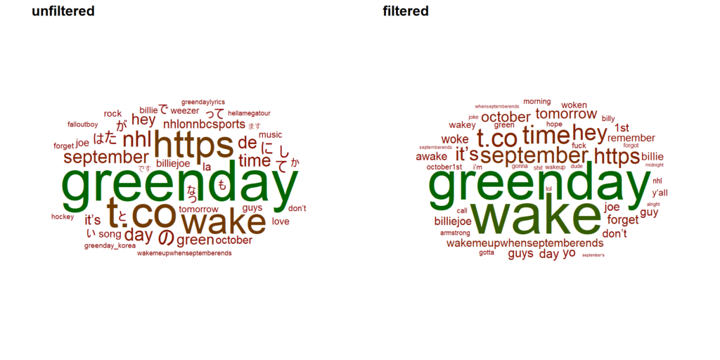
In the unfiltered dataset there seem to be some Korean signs, but for obvious reasons, these disappeared after filtering. Furthermore, from the filtered word cloud I could deduct that the word wake is way more popular than woke, so the lame joke is probably more often expressed in the present tense.
This means that for the rest of the data collection, we will use the following query:
“greenday wake”
But first, apply this exact same filter on the 2019 dataset:
greenday_2019 <- greenday_071019 %>%
  filter(str_detect(text, "wake"))

greenday_2019 %>%
    summarise(number_of_tweets = nrow(.),
            earliest_tweet = min(created_at),
            latest_tweet = max(created_at),
            number_of_unique_users = user_id %>% unique() %>% length() )
| number_of_tweets | earliest_tweet | latest_tweet | number_of_unique_users |
|---|---|---|---|
| 3200 | 2019-09-28 00:35:38 | 2019-10-07 19:02:17 | 3115 |
Figuring out how to collect earlier tweets
The next part in my quest to figure out how many people will joke about “waking up Greenday when September ends”, was to collect tweets from the September – October transition of the years prior to 2019. I could not use Rtweet’s search_tweets function because of its 9-day limit. For searching the full archive, I will need another function from the same package called search_fullarchive. Although the name of this function sounds extremely promising, I soon realised that it would not help me out of the box.
I discovered that apparently there are several limits to searching the complete Twitter archive. First, you need a developer account which has to be approved by Twitter. This was actually easier than I thought, but still some unforeseen hazzle. Next, I had to set-up a developer environment, stating what I was planning to do with my access to the Twitter archive. And finally, when all of this was done, I realised that the maximum number of searches I could do in one month was 50, with only 100 searches per query.
Let me do the math for you: This means that I would only be able to query for a maximum of 5 000 tweets a month! Given that my 2019 dataset contained around 3 200 tweets, this means that, if I am lucky, I would be able to extract data at a rate of 1 September-October transition per month. If you remember that this song was released in 2005, you will probably have figured out that it would take me around 13 months to gather all the necessary data, excluding 2019 because I already have that dataset. Boy, have I underestimated this task.
So what now? I browsed the web, wondered why I desperately wanted to continue this extremely irrelevant quest, told myself that I was already too deeply invested in it to stop now, realised I was talking to myself and then listed my options:
- Buy Twitter premium developer access for only $1 899 to get access to not 50 but 2 500 requests per month
- Implement the algorithm for bypassing the Twitter API restrictions published in this paper
- Use a scraping tool like Twint
- Slowly collect each year’s data by performing my 50 requests/month
I think I do not need to explain to you why I did not pay 1 700 euro for a handful of Twitter requests. But you might wonder why I did not go for option 2 and 3. Well, both of them are against Twitter’s terms of service as they actively circumvent their API. Since I am not that much of a badass and I do not want to be banned from the platform, I was left with only one single option: option number four. A slow, painfully long data collection process. Why not?
Data collection: earlier tweets
The goal here is to collect data between the exact same date interval as the 2019 dataset. This means tweets containing the words “greenday” and “wake” from 28/09 up until 08/10. I wanted to work my way back, so first up was the year 2018.
But first I defined a helper function, which was necessary to correctly feed in the dates to rtweet’s search_fullarchive function:
# Helper function
parse_date_time_for_rtweet <- function(date_time) {
  str_c(year(date_time),
        if_else(nchar(trunc(month(date_time))) == 2,
                as.character(month(date_time)),
                str_c(0, month(date_time))
        ),
        if_else(nchar(trunc(day(date_time))) == 2,
                as.character(day(date_time)),
                str_c(0, day(date_time))
        ),
        if_else(nchar(trunc(hour(date_time))) == 2,
                as.character(hour(date_time)),
                str_c(0, hour(date_time))
        ),
        if_else(nchar(trunc(minute(date_time))) == 2,
                as.character(minute(date_time)),
                str_c(0, minute(date_time)))
  )
}
The script below starts on the newest day (08/10) and, hopefully, worked its way back to the oldest day (11/09).
# Find 2018 tweets
min_time_parsed <- 201810080000

while (min_time_parsed > 201809280000) {

  # Do the search
  query <- search_fullarchive(q = "Greenday wake -from:GreenDay_Robot",
                              n = 100,
                              safedir = "full_search",
                              env_name = "development",
                              fromDate = "201809280000",
                              toDate = min_time_parsed
                              )

  # Find new max time
  min_time <- query %>% pull(created_at) %>% min()
  min_time_parsed <- parse_date_time_for_rtweet(min_time)

  # Add to dataset
  greenday_18 <- greenday_18 %>%
    bind_rows(query)
}
I did this search for the first time in October 2019 and as expected, I reached my monthly limit rather quickly. But I was hopeful. Maybe I somehow still managed to capture all 2018 tweets?
greenday_18 %>%
    summarise(number_of_tweets = nrow(.),
            earliest_tweet = min(created_at),
            latest_tweet = max(created_at),
            number_of_unique_users = user_id %>% unique() %>% length() )
| number_of_tweets | earliest_tweet | latest_tweet | number_of_unique_users |
|---|---|---|---|
| 1871 | 2018-10-01 15:40:23 | 2018-10-07 23:55:18 | 1841 |
Nope. I did not even make it into September. Worthless. With only data from 2019, half of the data from 2018 and no searches left on my developer account this month, I gave up.

Finally, it’s November. Now I can try again! I am going to spare you all the code and will just give you the summary table for the 2018 dataset:
| number_of_tweets | earliest_tweet | latest_tweet | number_of_unique_users |
|---|---|---|---|
| 5203 | 2018-09-28 00:54:45 | 2018-10-07 23:55:18 | 5069 |
VICTORY! By being somewhat patient, I obtained two years of data, ready to explore the popularity of this lame Greenday joke.
But what a minute? I did not get any errors reporting that I was over this month’s rate limit. Maybe I still have some queries left to squeeze out some of the 2017 data? I reran the script and summarised the 2017 data here:
| number_of_tweets | earliest_tweet | latest_tweet | number_of_unique_users |
|---|---|---|---|
| 2587 | 2017-09-28 04:10:00 | 2017-10-07 21:32:05 | 2518 |
What? This is crazy! Next to finishing the 2018 dataset, I was also able to extract almost all 2017 tweets, before reaching my November rate limit! Time to integrate all the datasets.
Popularity of tweeting about waking up Greenday in the September-October transitions of 2017, 2018 and 2019
Time for plotting!
# Combine all datasets
complete_dataset <- greenday_17 %>%
  bind_rows(greenday_18) %>%
  bind_rows(greenday_071019_filtered) %>%
  mutate(year = as.character(year(created_at)),
         month = month(created_at),
         day = day(created_at),
         hour = hour(created_at))

# First plot
complete_dataset %>%
  group_by(year) %>%
  summarise(number_of_tweets = n()) %>%
  ggplot(aes(x = year, y = number_of_tweets)) +
  geom_col() +
  coord_flip() +
  theme_bw() +
  ggtitle("Number of tweets about waking up Greenday from 29/09 to 08/10")
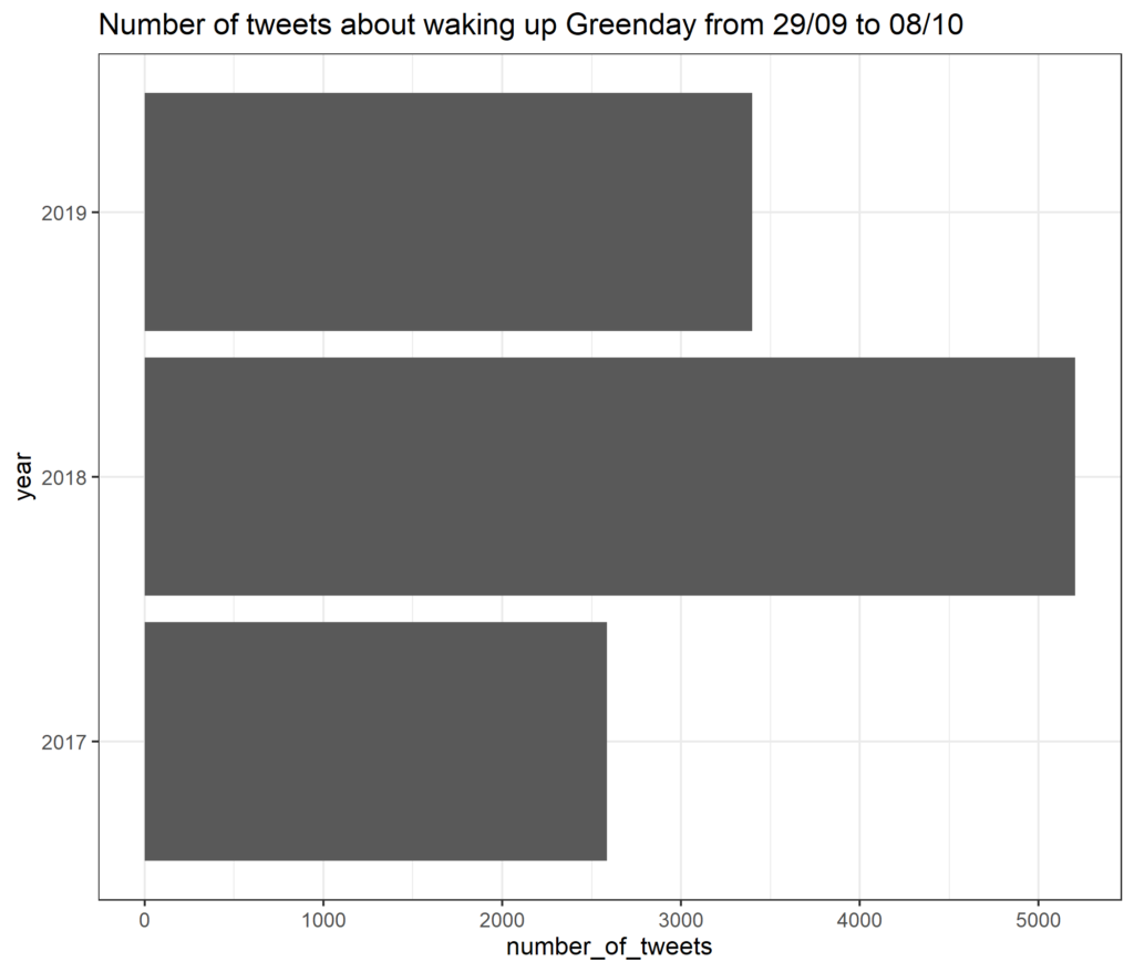
I am quite happy. Although the number of tweets containing a “WaKe GrEenDaY Up”-joke severely increased from 2017 to 2018, they did decrease again in 2019. Here’s another way of looking at this data:
complete_dataset %>%
  group_by(year, month, day, hour) %>%
  summarise(count = n()) %>%
  mutate(fake_date = ymd_hm(str_c("1991-", month,"-", day," ", hour, ":00"))) %>%
  ggplot(aes(x = fake_date, y = count, colour = year)) +
  geom_line(alpha = 0.8, size = 2) +
  ggtitle("Number of tweets about waking up Greenday from 29/09 to 08/10") +
  ylab("Number of tweets") +
  xlab("") +
  theme_bw() +
  scale_color_brewer(palette = "Dark2") +
  facet_wrap(~ year, nrow = 3)
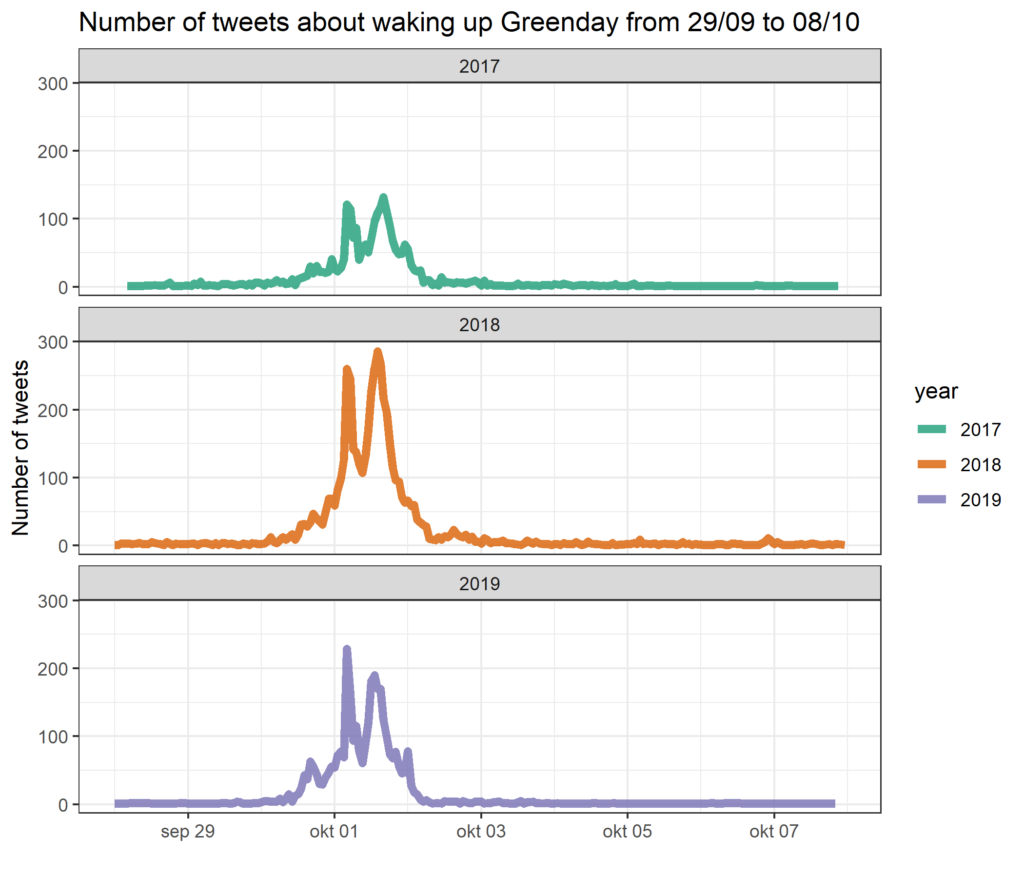
Cool! Each year clearly shows a very similar pattern, with two main peaks on the first of October. This is probably a result of different time zones waking up and being active on Twitter. Furthermore we learn that more and more people start tweeting about this joke from September 30th, with a more pronounced peak in 2019 compared to the other two years. Similarly, the 2017 and 2018 data show a longer tail with still some activity during October 2nd, which is less pronounced in the 2019 data.
Conclusions
First, searching Twitter using the R-package Rtweet is great if you would like to pick up trends from the last 9 days. However, due to the limitations set by the Twitter API, any user that does not have access to a premium account will have trouble retrieving older tweets.
Second, regarding my research question “how many tweets are sent out with this lame joke about waking up Greenday after September ended?”, I was able to get some insights in the data of the years 2017 – 2019. It is a little bit assuring that in 2019 less tweets were sent out compared to 2018, but having data from only 3 years does not give me a complete picture of the reality. I probably need to find other data sources. Stay tuned for next year because I have a few other ideas in mind. (Please remind me next September on Twitter to look into those).
Third, maybe, just maybe, I need to stop pursuing these stupid ideas and invest my time in something useful.
Maybe.