At the end of May, I was happy to hear that my second first-author paper, entitled Carrot juice fermentations as man-made microbial ecosystems dominated by lactic acid bacteria was published in Applied and Environmental Microbiology. I’m especially proud on this manuscript as we used different molecular (DNA vs RNA based 16S sequencing), analytical (HPLC-RI and HPAEC-PAD) and bioinformatical (DADA2 processing and phylogenetic placement) techniques. In addition, this paper was based on data which we obtained from our citizen-science project, Ferme Pekes. We launched this project 2.5 years ago by asking 40 different people from the Antwerp region (Belgium) to ferment their own carrots at home and bring in samples at regular time points. We got quite some press coverage for this project at that time, which was a plus as communicating your science to a broader audience really makes you rethink everything you’re doing in the lab.

While the carrot juice manuscript was the first one that I started writing, it wasn’t the first one that got published. That honour goes to our Lactobacillus casei group paper, which I co-authored with Stijn Wittouck and was published last year (more about that in a previous blog post). That means that I’m now main author of two papers. Two papers also means that they can be compared. And comparing things has become one of my specialities, the last few years.

Therefore, in this blogpost I will present to you my first comparative paperomics approach!

Metadata analysis

One of the first things I learned when writing scientific manuscripts was labelling different versions. This is extremely useful in the case you have to retrieve certain parts that you had to delete for “word limit” or “This might be interesting but is irrelevant for the story now”-reasons. I always labelled my files using the ‘DATE_MANUSCRIPTNAME_LASTEDITOR.docx’ format. My manuscript folder then ends up looking something like this:

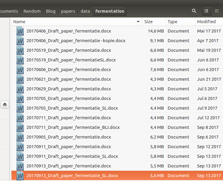
Currently, I’m writing my PhD thesis in LaTeX, but these two manuscripts were drafted in Microsoft Word and/or LibreOffice. This, together with my labelling strategy, led to many different “.docx” and “.odt” files. While I love writing in LaTeX, I’m actually quite happy that I wrote these papers in Word/LO, as a lot of extra metadata is stored within these file formats. And it’s that metadata that I’ll be using here to perform my comparative paperomics!

Data collection

A Word document is basically a .zip file that contains your main text and several other files it needs for formatting. To extract the data I’m interested in, I wrote a small bash script that unzips every “.docx” file and copies the “app.xml” file from the unzipped docProps folder:

 

 

 

https://gist.github.com/swuyts/ae022435c3fdff6552bcb8b50a4ab089

Now for each version I’ve ended up with a .xml file that looks like this:

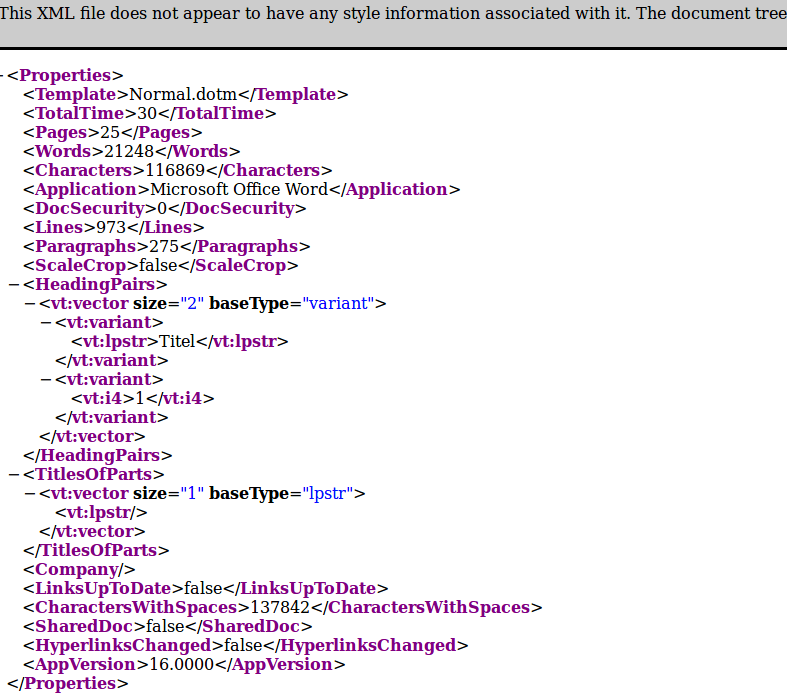
The next step is of course data extraction from these xml files, and for this I will be using (can you guess?)…

R!

 

 

https://gist.github.com/swuyts/5562cfce96e01956df798a0074166896

Analysis

All right, we got our data! Let’s explore this dataset by plotting some of the variables:

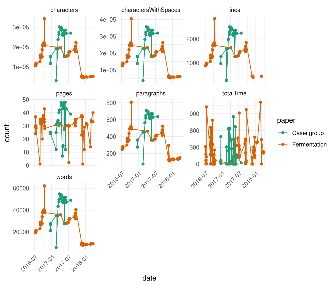
A lot of information all at once! But a quick glimpse to the shape of the different plotted parameters reveals that most of them are highly correlated. For example, characters, charactersWithSpaces, lines, paragraphs and words, all show almost the exact same shape. Furthermore, this graph clearly shows that the timespan where we worked on the Fermentation manuscript (orange) was way longer than the timespan of the Casei group manuscript (green). This is due to a lot of reasons, but the main one being that for the carrot juice fermentation paper we needed to perform a lot of extra wet lab experiments to answer novel questions that were raised during the drafting of the manuscript, while with the Casei group paper, things went a little bit smoother.

This is also reflected if we sum up and plot the totalTime edited per paper:

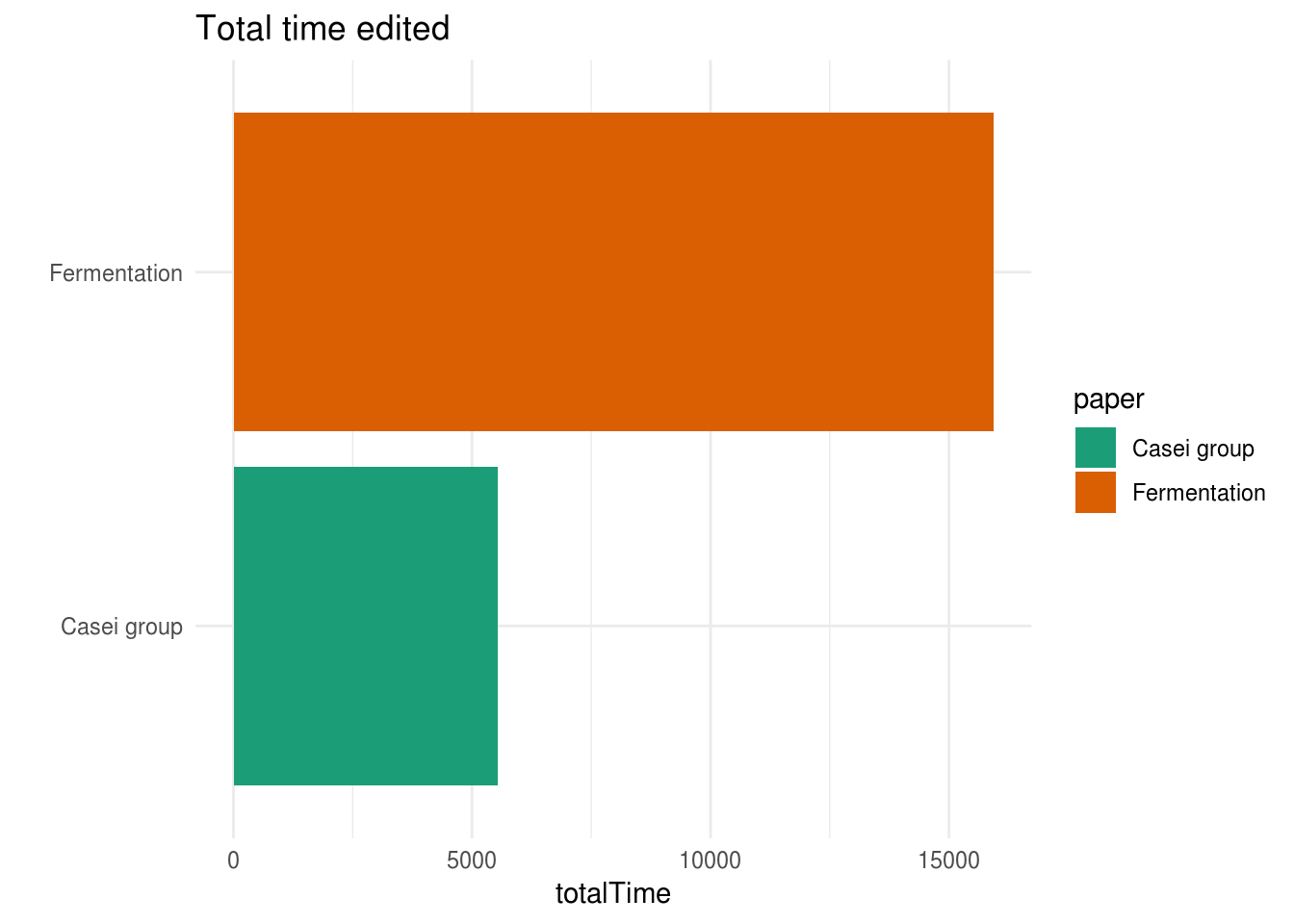
I’m guessing that the totalTime variable shows the amount of minutes worked on this document. I’m not sure how trustworthy the timer of Microsoft Word is, but there’s definitely a clear difference between the two manuscripts. This difference might be caused by the fact that we have a lot more different versions for the Fermentation paper, compared to the Casei group paper. But, what if we pretend that these numbers are real, that means that we’ve spent a total of 3.8 days on writing the Casei group manuscript, while the Fermentation manuscript took slightly more than 11 days!

In a next step, let’s have a short look at the number of words that were written.

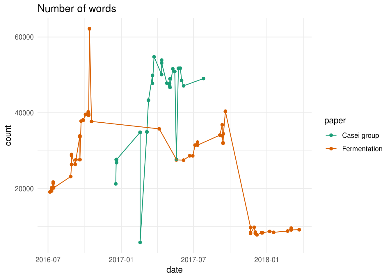
This graph shows the pain of every PhD student (and author in general): writing a big chunk of text, that has to be deleted later on. While this graph is probably biased by the text written in comments, it does show two drastic reductions in the number of words for the Fermentation manuscript. The most pronounced one is the one near the end of 2017, when we were preparing the manuscript for submission.

However, I’m a bit surprised by the difference in final word count between both papers. It seems unlikely that the Casei group paper has that many words compared to the carrot juice fermentation paper, especially as the official word count we provided to the journals were 5321 and 5533, respectively. I’m not sure what causes the high number of words in the Casei group paper but my guess is that something went wrong with the formatting of the references. Better quality control should probably fix this problem.

Text mining

The metadata analysis already revealed some unexpected patterns. But I’d like to dig a little bit deeper and look at the raw data: the words we’ve written!

Data collection

Data collection is a little bit easier here. For this analysis I’ve copy pasted the last version of each manuscript into a ‘.txt’ file and imported that into R to analyse it with the awesome tidytext package!

 

https://gist.github.com/swuyts/d5429770e91fe854b6ea67621cba07e0

Analysis

Now that we have our dataset ready, it does not take a lot of effort to look at the most frequent words per paper. Let’s start with the Casei group:

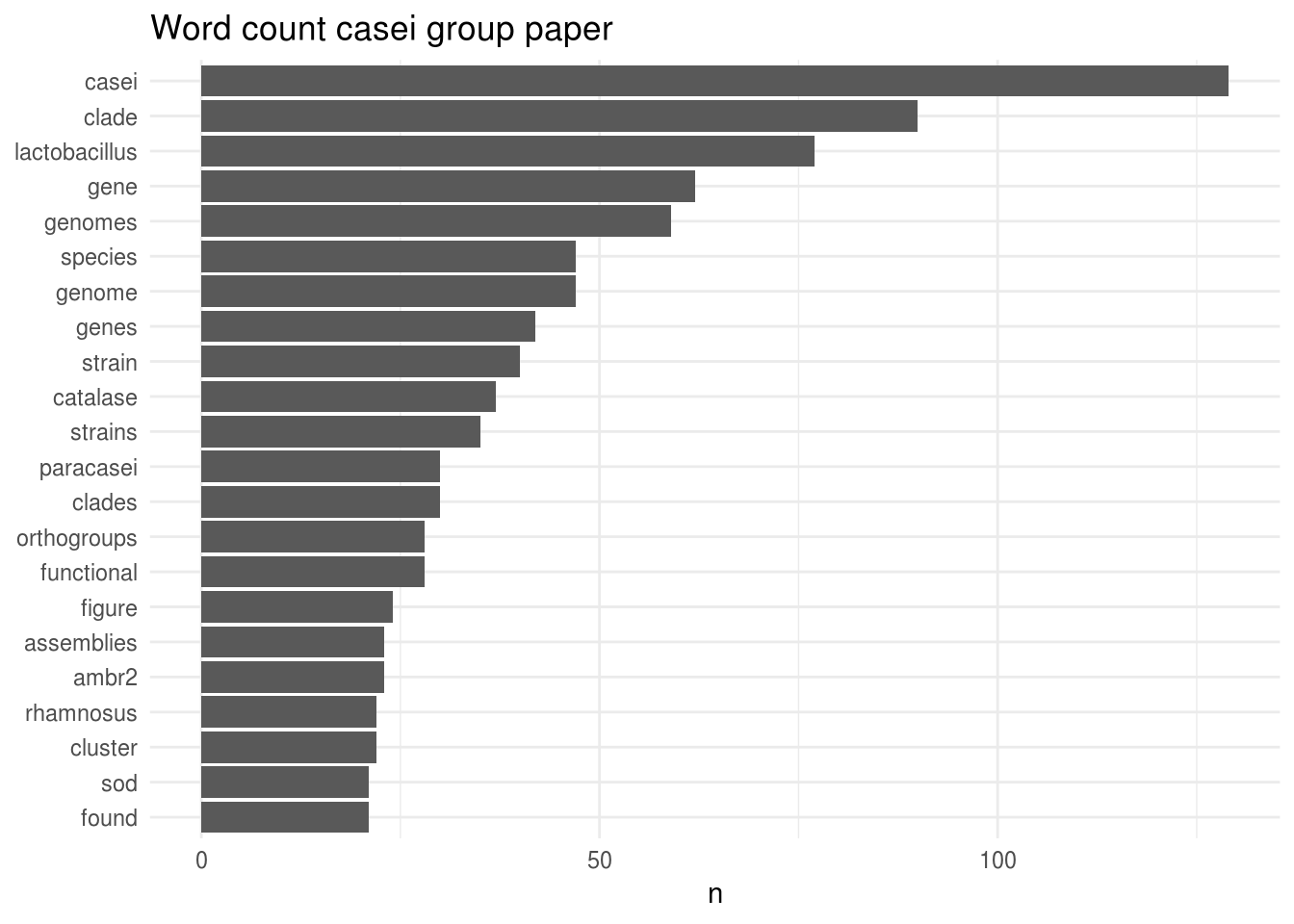
Well, that’s not a surprise: casei is by far the most used word in this manuscript. It is followed by the word “clade”, which is also not surprising for a phylogenomics manuscript.

What about the fermentation paper?

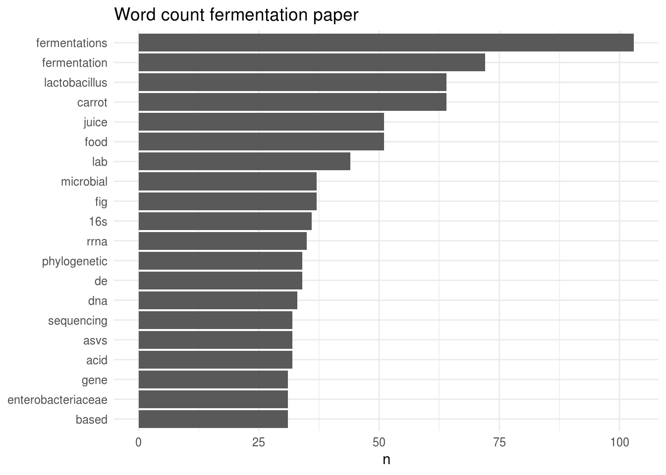
Well, the graph speaks for itself… This manuscript clearly talks a lot about fermentations, fermentation, Lactobacillus, carrot and juice.

I must admit, the most frequent word count does not really provide a lot of interesting insights. But what if we look at the most common pair of words?

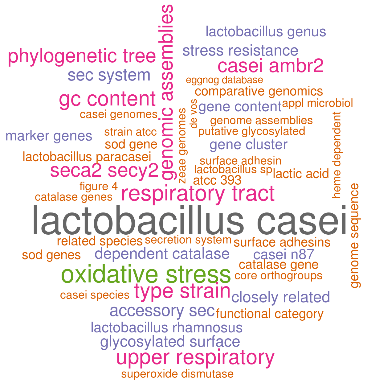
This is already a little bit more interesting! Besides the wordpair Lactobacillus casei, the most common combination of words is “oxidative stress”“, one of the main topics we handle in the paper. Other examples include ”casei ambr2″ which is a strain we isolated from the “upper respiratory tract” and heavily discuss in this manuscript. Or “seca2/secy2”, which is the putative role of an interesting gene cluster we described.

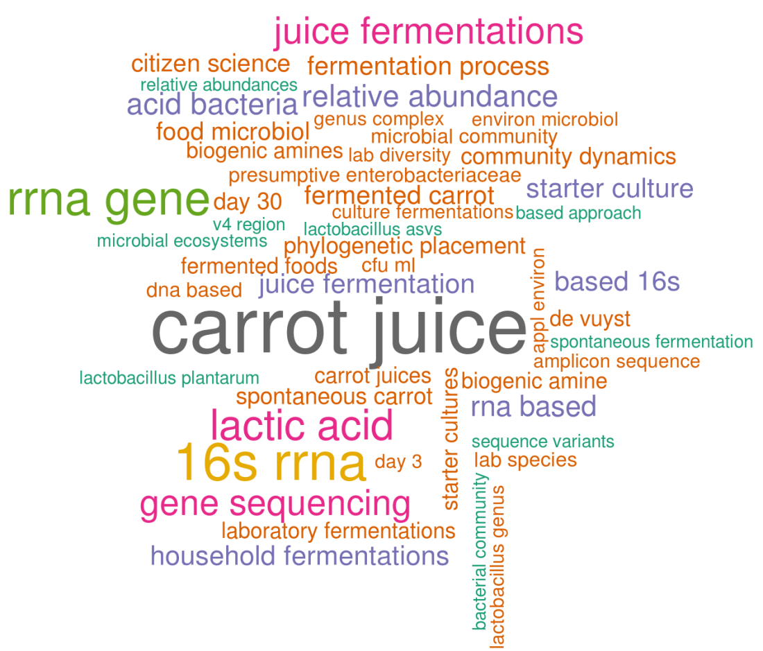
What about the carrot juice fermentation paper?

In this manuscript, “carrot juice” is obviously the most common word pair. It is followed by 16S rRNA which is the main technique (16S sequencing) we used to study the fermentation process. Other things that caught my eye are “phylogenetic placement”, a technique we used to place our ASVs (~OTUs) on a phylogenetic tree or biogenic amines, a group of molecules that can cause nausea if they are too abundant in a fermented food product, which we also measured. In general, this wordcloud looks like a good graphical summary of our recent manuscript!

Conclusion

The field of comparative paperomics is still young. Many different computational methods will need to be developed to support this great new promising -omics technology, especially for quality control. Nevertheless, in this proof of concept we’ve showed that i) I’ve authored two publications on which I’m very proud, ii) the fermentation manuscript took much longer to draft than the casei group manuscript for various reasons and finally, iii) using text mining we were able to get some preliminary insights into the content of these papers.

Alternatively, one could also go an read the abstracts, which will probably contain a lot more useful information than this blog post, here and here.

Thanks for reading, see you next time!

The full pipeline can be found as a RMarkdown file on my Github page.